# `kortical.features.time_series`

# Introduction

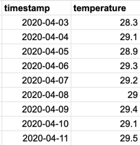
Time series data is a collection of measurements of one or more values over time. Consider the following dataset of daily temperature:

In most cases we wouldn't use this data directly for machine learning because each row only contains information about temperature at this point in time. There are many reasons this isn't helpful:

For lots of time series problems, the value of variable X right now is only part of the story - we need to understand variable X in relation to various norms such as moving averages.
The sample frequency (or time granularity) we are interested in might be different to that in the timestamp, for example we could be looking to model longer term trends and therefore might want to consider temperature in terms of the weekly average.
The target we are trying to predict is often some point in time in the future (e.g. the temperature next week), so won't be available at this time stamp.

To address these problems, we need to transform the original dataset into a set of observations suitable for machine learning. For example:

Here, we have inserted some columns: aggregated temperature over a specific time window (the rolling average temperature over the last 7 days), a delta (the difference betweeen today's temperature and the rolling average), and finally a target column for prediction purposes (the temperature tomorrow). In reality, we would create many more columns, varying both the time window (e.g duration, offset) and aggregation function (e.g max, standard deviation) to better describe the behaviour of our target.

There is not a one-size-fits-all answer for creating these windows, especially when there are domain-specific aspects involved. For that reason, it is desirable for you to be able to iterate quickly and test various hypotheses on size, number of windows, time granularity and sometimes even target to find the best fit for your problem. The Kortical time series package is designed to accelerate this process.

# Realistic Usage

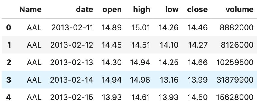
In the real world, time series data tends to have multiple variables we care about at each time step, and we might need to aggregate these in multiple ways over multiple window sizes at a given sample frequency. For example take this stock data (you can download this dataset here):

In this dataset we can see daily measurements for multiple values such as opening price (open), closing price (close) and volume. There is also a field called Name - this contains the stock symbol, and indicates to us that there are multiple entities of interest in this time series.

The below code shows a typical transformation using the Kortical time series package:

from datetime import timedelta
import pandas as pd

from kortical import datasets
from kortical.features import time_series as ts
from kortical.features.time_series import Functions as fns

# Use example data (available in Kortical SDK)
df = datasets.load('stock_prices')

rows = ts.create_rows(
    dataframe=df,
    
    # Set the datetime index of this data
    datetime_column='date',
    
    # Column(s) containing unique subsets whose time series must be treated differently. String or list of strings.
    id_columns='Name',
    
    # Columns which require aggregating (i.e measurements).
    columns=['open', 'high', 'low', 'close', 'volume'], 
    
    # Specify time windows (i.e vary lag/duration)
    time_windows=ts.lags_daily_over_10_days + ts.lags_weekly_over_3_weeks + ts.lags_monthly_over_3_months + ts.lags_yearly_over_3_years,
    
    # Aggregation functions; these must accept a list and return a scalar.
    functions=(fns.mean, fns.std, fns.min, fns.max),
    
    # Resample over days instead of hours (i.e adjust time granularity).
    sample_frequency=timedelta(days=1),
    
    # Describes how to read date strings in the df. 
    datetime_format='%Y-%m-%d')

# Finally, index by datetime
rows.index = pd.to_datetime(rows.index).date

The output of this is a table which still has a row for each stock on each day, but instead of just listing raw measurements (high, low, volume etc.), it contains a grand total of 231 features! After transformation, the rows are embedded with lots of historic information, which will help a machine learning model make better decisions:

Before we can use these rows for prediction tasks, we need to add a target:

# Example continued from above...

rows['close_tomorrow'] = rows.groupby('Name')['close_window0'].shift(1)
rows.dropna(subset=['close_tomorrow'], inplace=True)
rows['close_tomorrow_higher'] = rows['close_tomorrow'] > rows['close_window0']
del rows['close_tomorrow']

This code snippet uses pandas' .shift() method to create a new column close_tomorrow_higher, which is True if the closing price of this stock tomorrow exceeds that of today's.

We are now ready to upload our dataset to the platform for machine learning.

#

# Time Windows

As we saw in the previous section, a key part of the transformation is choosing a selection of time windows over which to perform our aggregations. A time window is defined by its duration and offset. The time series library offers the following options by default:

lags_daily_over_10_days
lags_weekly_over_3_weeks
lags_monthly_over_3_months
lags_monthly_over_6_months
lags_yearly_over_3_years
lags_daily_over_10_days_last_year
lags_weekly_over_3_weeks_last_year
lags_default_daily (equivalent to lags_daily_over_10_days + lags_weekly_over_3_weeks + lags_monthly_over_3_months)
lags_default_monthly (equivalent to lags_monthly_over_6_months)

You can easily create your own time windows by using one of the provided generator functions. Calling one of these will return a smaller section of adjacent measurements from the original time series. Examples:

from dateutil.relativedelta import relativedelta
from kortical.features.time_series import generate_daily_windows, generate_weekly_windows, generate_monthly_windows, generate_yearly_windows

# For every day, extract a window (5 days long) 
lags_daily_over_5_days = generate_daily_windows(num_days=5)

# For every week, extract a window (12 weeks long, offset by 1 year)
lags_weekly_over_12_weeks_last_year = generate_weekly_windows(num_weeks=12, start_offset=relativedelta(years=1))

# etc...

For full control over time window creation, use the TimeWindow class.

# Full documentation

# `create_rows`

This function transforms time series data into a format that is more suitable for machine learning. Time windows and aggregate functions are used to create features and targets, which lead to better model performance in the Kortical Platform.

Inputs

dataframe - input dataframe.
datetime_column - the column which has the datetime index.
columns - the column(s) which vary over time (i.e "measurements"); string for single column, list for multiple columns.
time_windows - time windows to apply to the columns.
functions - aggregate functions to apply across time windows. This must accept a list of numeric values and return a scalar.
sample_frequency - how often to create an observation (e.g daily, monthly, weekly) as time delta.
datetime_format (= None) - the format of the datetime values in datetime_column, defined in terms of the directives described here (opens new window). If not provided, uses pandas.to_datetime() to infer the format. Performance can be significantly better if the format is explicitly provided.
id_columns (= None) - ID(s) to differentiate between different time series objects.
resample_rule (= None) - resample rule passed to pandas.DataFrame.resample().
resample_aggregations (= None) - resample aggregations passed to pandas.DataFrame.resample().agg()
ignore (= IgnoreTimeComponent.HOUR) - if you need to ignore part of the time component, specify that here. Acceptable arguments are IgnoreTimeComponent.NONE, IgnoreTimeComponent.HOUR, IgnoreTimeComponent.MINUTE and IgnoreTimeComponent.SECOND.

Returns

df - dataframe containing the generated rows.

from kortical.features.time_series import create_rows

rows = create_rows(
            dataframe,
            datetime_column,
            columns,
            time_windows,
            functions,
            sample_frequency,
            datetime_format=None,
            id_columns=None,
            resample_rule=None,
            resample_aggregations=None,
            ignore=IgnoreTimeComponent.HOUR)

# `Functions`

This class contains a range of typical aggregation functions that may be applied to time windows.

Inputs

list - A list of numerical values (e.g time series measurements)

Return

float - A single numerical value.

from kortical.features.time_series import Functions

function_1 = Functions.max     # Returns the maximum value
function_2 = Functions.min     # Returns the minimum value
function_3 = Functions.sum     # Returns the sum of all values
function_4 = Functions.mean    # Returns the mean of the values
function_5 = Functions.median  # Returns the median of the values
function_6 = Functions.std     # Returns the standard deviation of the values

# `TimeWindow`

This class gives you full control over the creation of time windows, and should only be used when a desired time window cannot be imported or created with the provided generator functions (see the section Time Windows).

Input

start - the start time delta, either relative to the start of the series or an absolute time.
duration - the duration of the time window or an absolute time.
offset (= None) - to add a fixed time offset, add that here.
use_value_as_is (= False) - do not apply functions to the data within this time window; instead, just copy the first value in the window to the result. Intended to be used with daily lags where it doesn't make sense to apply functions to a single daily value.

Return

TimeWindow - a TimeWindow object.

A simple usage example is given by looking inside our generate_daily_windows() function:

from datetime import timedelta
from kortical.features.time_series import TimeWindow

def generate_daily_windows(num_days, start_offset=None):
    start_offset = start_offset if start_offset else timedelta()
    return [
        TimeWindow(
            start=start_offset + timedelta(days=i),
            duration=timedelta(days=1),
            use_value_as_is=True
        ) for i in range(num_days)
    ]

Note

The TimeWindow object should always be used inside a function such as this one; this generator function may then be used to create a time window that can be passed into time_series.create_rows.

← Feature Engineering Anonymization →

# kortical.features.time_series