# Evaluation Metrics
Once we have trained an ML Solution (which encompasses feature transformation, feature creation
and our trained model), we want to know how well it predicts the target outcome. A target could
be a real number, making our problem a regression problem, or it could be one or more of a discrete number of outcomes, which is a
classification problem.
The appropriate way to measure the success of our prediction depends not just on if we are evaluating a
regression or classification problem, but also on the properties of the problem itself.
For example, a common evaluation metric for classification tasks is a simple accuracy score,
which is easy to understand and explain to the non-technical but has the undesirable property of giving misleading scores
in situations where classes are imbalanced (see here for details).
In general the evaluation metric you choose should relate to the real world problem you are trying to solve so there is never a one size fits all, and its not possible for us to know just from your data which would be the most appropriate.
# Evaluating Classification Tasks
A classification task involves predicting if a target belongs to set of given options. There are several flavours of
classification task, which have an impact on which evaluation metric may be more suitable:
binary classificationis one of the most common kinds of problem and is where a target can only have one of two potential states. An example of this would be predicting if a customer will unsubscribe next month.multiclass classificationis where our target can have one of a finite number of states. An example of this would be predicting the best offer type to send a customer.multi-label classificationis where our target can haveNof of a finite number of states (potentially more than one correct answer). An example here might be predicting the tags to append to a document.
There is no hard and fast rule as to which kinds of evaluation metric are suited to which kind of classification task,
with the exception that Mean Average Precision @ K really only makes
sense for multi-label classification as it is designed to handle multiple correct predictions.
# Accuracy
Accuracy is simply the fraction of predictions our model got correct.
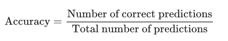
This is very easy for a non technical user to understand but is only really interpretable where you have a balanced number
of classes. If, for example, you have a binary classification problem where the positive case only appeared in 5% of
observations, a model which simply predicted 0 for everything would get an accuracy score of 95%!
Pros:
- Easy to understand and to communicate (very important in some cases)
Cons:
- Loses meaning in cases where classes are imbalanced (as they will be in a vast majority of real world problems)
# Area Under the ROC Curve
Taking the crown as both the hardest to communicate and potentially most useful evaluation metric, Area Under the ROC Curve
(also commonly known as just AUC or roc_auc) is a measurement of classification performance where the worst possible score
is .5 and the best is 1.
Uniquely among the other score types here it is not dependent on the chosen classifier threshold. It is also reasonably robust to imbalanced data, which makes it a great initial first choice for getting started on binary or multi-class problems. It is also scale invariant, measuring how well predictions are ranked regardless of their absolute values.
AUC score is derived from examining a classifiers True Positive Rate (aka TPR or recall) vs False Positive Rate (FPR) tradeoff
across a range of potential classifier thresholds.
True Positive Rate is given by:
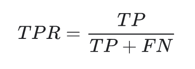
Where False Positive Rate is given by:
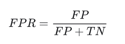
and
TP=number of true positivesTN=number of true negativesFP=number of false positivesFN=number of false negatives
The above equations require a choice of classifier threshold to evaluate (with higher classifier thresholds leading
to lower False Positive Rates and lower thresholds leading to lower False Negative Rates). If we evaluate these equations
over a range of possible thresholds, we get a curve describing how these tradeoffs change, known as an ROC
curve:

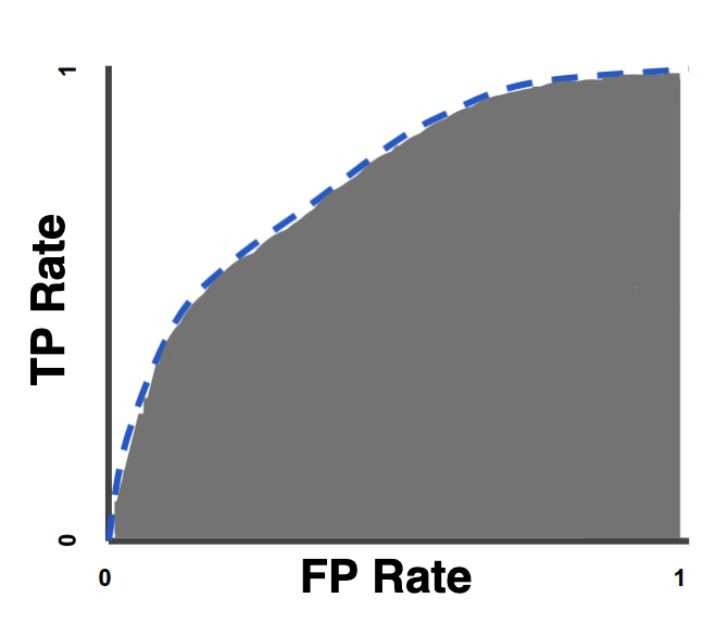
To calculate the Area Under the ROC Curve, we simply measure the area under this curve!
Pros:
- Classifier threshold invariance - will give a stable prediction of classifier quality regardless of the chosen threshold.
- Scale invariant - measures how well predictions are ranked regardless of their absolute values, great for problems where we care about the output ranking being accurate rather than estimates of probability.
- Works well with imbalanced target observations.
Cons:
- Hard to explain and interpret in of itself (aside from knowing higher is better!).
- In cases we care about well calibrated probability outputs it's scale invariance is not a useful property.
Fun Fact
The ROC part of the acronym stands for Reciever Operating Characteristic and is so called due to early radar systems (opens new window)
# F1-Score
F1-Score is the harmonic mean of the precision (opens new window) and the recall (opens new window) and is a good proxy for accuracy in cases where we have class imbalance. Its easier to communicate to the non technical than AUC, while still having the desirable property of robustness to class imbalance.
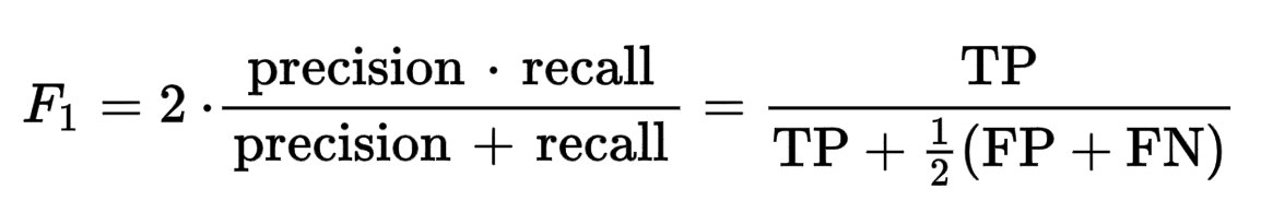
Where:
TP=number of true positivesFP=number of false positivesFN=number of false negatives
Pros:
- Takes into account absolute output probabilities, in situations this is important (unlike AUC).
- Easy(er) to describe to clients than metrics AUC or Logistic Loss.
- Outputs a score between
0and1where1is best, which helps with intuitive understanding. - Handles class imbalance.
- Good for imbalanced multiclass problems.
Cons
- Relies on choice of classifier threshold.
- Doesn't take true negatives into account so unsuited for certain binary problem types.
# Log Loss
Log Loss (or Cross-entropy loss), measures the performance of a classification model whose output is a probability value
between 0 and 1. You can think of Log Loss as minimizing the distance between two probability distributions - predicted and actual.
The derivation is rather complex so please refer to this (opens new window) article to see the full formula.
Cross-entropy loss increases as the predicted probability diverges from the actual label. So predicting
a probability of .012 when the actual observation label is 1 would be bad and result in a high loss value. A perfect model
would have a log loss of 0.
Pros:
- Good for when we care about the output probabilities being correct more than the relative ranking.
Cons:
- Hard to interpret and explain
- Some users might find a classification metric where
0is the best possible score counterintuitive. - Not useful when we care more about relative ranking rather than absolute probabilities
# Mean Average Precision @ K
Mean Average Precision @ K (aka MAP@K or MAP@N). This metric is for multi-label problems. For brevity, we won't go
into the full detail here but recommend this (opens new window)
article to fully explain the metric.
In essence though, in situations where we have a multiple set of correct answers
for each observation, MAP@K, looks at the average precision (opens new window)) across
the top K choices, ignoring the rest.
You can use this metric by replacing K with your cutoff in the spec, for example if we want K to be 4, we could write the following:
  - data_set:
    ...
    - evaluation_metric: mean_average_precision_at_4
    ...
Pros:
- Suitable for the case where we only care about the top
Kpredictions the model makes, such as with recommender systems.
Cons:
- Very complex to interpret
- Only really useful for multi-label problem types
# Evaluating Regression Tasks
A regression task is where we have a target which is a real number and that can have, at least in theory, and infinite set of
possible values. The evaluation metrics we have for regression tasks fall into two categories:
- R Squared and Explained Variance in which
the best possible score is
1, with lower scores being worse. - Mean Squared Error and Mean Absolute Error in which the
best score would be
0, with higher scores being worse.
As with classification, the real world problem dictates which metric to use. For example, if you wished to penalise outliers
to a greater extent, you might wish to choose Mean Square Error over Mean Absolute Error.
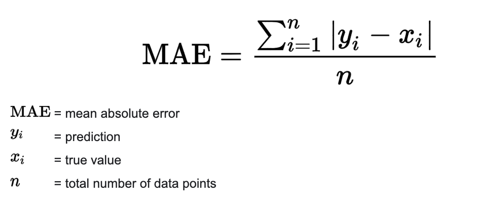
# Mean Absolute Error
Mean Absolute Error (MAE) is one of the simplest error metrics for regression tasks. For each observation, simply take
difference between the predicted value and the target value and then take the average of this over all observations.
Pros:
- Very simple to describe to end users.
- Useful for when the actual units of error are important to measure (eg if we wanted to know how much money we would make on a set of trades).
Cons:
- Only penalises the magnitude of the error linearly to the size, which is not desirable when you wish to penalise outliers
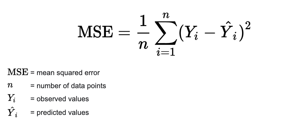
# Mean Squared Error
Mean Squared Error (MSE) is another extremely common error metric, and is simply MAE but
with a squared term before we take the average. This has the effect that outliers are penalised to a greater extent than with
MAE.
Pros:
- Provides additional penalties to outliers, useful for many kinds of problem where outliers are particularly undesirable.
Cons:
- Output units not directly interpretable, unlike with MAE.
- Can produce really big output numbers, which has implications for ease of visualisation.
# R Squared
R Squared (aka R2 or Coefficient of Determination) represents the proportion of variance that has been explained by the independent variables in the model. It provides an indication of goodness of fit and therefore a measure of how well unseen samples are likely to be predicted by the model, through the proportion of explained variance.
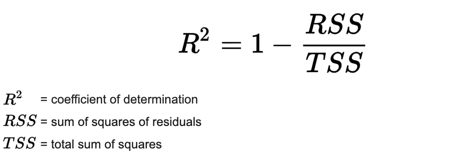
It is often in the range 0 to 1 although while 1 is the maximum, the minimum may be below 0.
Pros:
- Being between
0-1(in most cases) allows quick interpretation of how good a model is without needing to understand the underlying unit of measurement.
Cons:
- The fact that it is between
0-1in most cases can lead to confusion when this is not the case! - Doesn't have the same penalty for outliers as with
MSE. - Can be misleading since the variance is different between different datasets, which effects the scaling.
# Explained Variance
Very similar to R2 (actually identical if the mean residue is zero), explained variance is given by
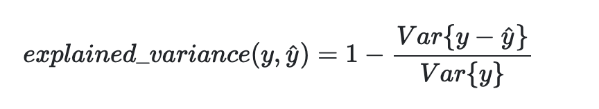
where yhat is the estimated target output, y is the corresponding (correct) target output, and Var is the Variance,
the square of the standard deviation.