# Models
Kortical, when left on its default settings, will attempt to create an appropriate machine learning solution to maximise ability to predict your target on unseen data. This solution may consist of a single model or an encoder step such as Word2Vec combined with a model.
The vast number of potential solution configurations possible is automatically and intelligently searched through as part of the Kortical AutoML process. This means a beginner user can just use the default settings and expect to get a powerful machine learning solution to be created for them (assuming sufficient observations in the dataset to support the complexity of the chosen target).
Advanced users are able to adjust the default list of model types and parameters, by using the Kortical language. High level information around the models available are contained below.
# Model types
Kortical supports all the key families of machine learning models we find are the best in class for solving problems today:
The default set of model types in the platform is:
  - models:
    - one_of:
      - xgboost
      - linear
      - random_forest
      - extra_trees
      - decision_tree
      - deep_neural_network
      - lightgbm
These are used in conjunction with one or more of the available text embeddings if there are text columns available:
  - word2vec
  - glove
  - tfidf
We don't include SVMs by default for a number of reasons. The veteran data scientist
may include them by simply adding them to the existing list:
  - models:
    - one_of:
        - SVM
We appreciate that this doesn't represent the complete universe of machine learning approaches - however we have curated this shortlist by benchmarking almost all available best-in-class models against a large set of academic, Kaggle (opens new window) and proprietary datasets. We find that almost without fail, the best model found for the problem belongs to one of our shortlist.
Note
We are always looking to make our platform better - if you know of an open source model you have found effective, we are happy to add it to the platform provided it outperforms our existing selection in our benchmark - just contact support.
# Decision Trees
Decision Trees (DTs) (opens new window) are a non-parametric supervised learning method used for classification and regression. They are quick to train and to predict, but tend to overfit, have large variance as small changes in the input data can result in very different trees and they can't represent complex problems.
Their main utility tends to be giving a quick baseline model on very large datasets. They are also used as the weak learners in Forest model ensembles.
Available Parameters: Decision Tree Classifier
- decision_tree:
  - criterion
  - splitter
  - max_features
  - max_depth
  - min_samples_split
  - min_samples_leaf
  - min_weight_fraction_leaf
  - max_leaf_nodes
  - min_impurity_decrease
  - class_weight
  - presort
Available Parameters: Decision Tree Regressor
- decision_tree:
  - criterion
  - splitter
  - max_features
  - max_depth
  - min_samples_split
  - min_samples_leaf
  - min_weight_fraction_leaf
  - max_leaf_nodes
  - min_impurity_decrease
  - presort
Take Care
With each algorithm we have a slightly different set of parameters between the Regressor and the Classifier.
# Forests
Forest models are independently trained ensembles of decision trees, trained on sub-samples of the dataset, using averaging to improve the predictive accuracy and control over-fitting.
# Random Forests
Random Forests (opens new window) are an array of parallel decision trees which vote together to produce a prediction. The method usually works better than an individual decision tree, as while each constituent decision tree might be biased in some way, a sufficient number voting together will have the effect that the individual biases cancel each other out and one is left with an accurate prediction of target signal.
Prior to the rise of Gradient Boosting Machines such as XGBoost, Random Forests were one of the most popular algorithms in competitive prediction tasks. They are still popular as a baseline model today, as they have the desirable property of being relatively good on most problems with the default parameters. That being said, they can still be the best choice available, outperforming other machine learning algorithms on certain types of dataset.
Random Forests have the following benefits:
- Robust to outliers.
- Work well with non-linear data.
- Lower risk of overfitting than individual Decision Trees and other models.
- Runs efficiently on a large datasets (although not as efficiently as Gradient Boosting Machines).
- Tends to generally work well on most problem types - not hugely sensitive to parameter choice
But with these comes some downsides:
- They can be biased while dealing with categorical variables.
- Can be slow at training compared to some other approaches.
- Not suitable for datasets with a lot of sparse features (e.g. high cardinality categorical or TF-IDF text fields).
- Creates a non-smooth decision boundary
What's a non-smooth decision boundary and why do we care?
Imagine you are building a model to predict if a customer will accept a quote, based on properties like quantity and margin.
Your end application will permutate these input variables to find the optimal quote. If you use a model with a non-smooth
decision boundary for such an application, you will find that small changes in input may not cause any change in output, or that
a small change in input causes a big step in the output probability with no intermediate steps.
Choose a linear or deep_neural_network model type for smooth decision boundaries.
Available Parameters: Random Forest Classifier
- random_forest:
  - n_estimators
  - criterion
  - max_features
  - max_depth
  - min_samples_split
  - min_samples_leaf
  - min_weight_fraction_leaf
  - max_leaf_nodes
  - min_impurity_decrease
  - bootstrap
  - class_weight
  - oob_score
Available Parameters: Random Forest Regressor
- random_forest:
  - n_estimators
  - criterion
  - max_features
  - max_depth
  - min_samples_split
  - min_samples_leaf
  - min_weight_fraction_leaf
  - max_leaf_nodes
  - min_impurity_decrease
  - bootstrap
  - oob_score
# Extremely Randomized Trees
Extremely Randomized Trees (Extra Trees) (opens new window) are similar to Random Forests, but with added, controllable, randomness where each selected split in the current tree is the best split among a set of random uniform splits. This leads to the property that each tree is in itself less accurate but equally less likely to be overfitted, providing an overall difference in the bias-variance tradeoff (opens new window) compared to a conventional Random Forest.
The pros and cons of Extra Trees match those of Random Forests quite closely, with the key difference being that Extra Trees are cheaper to compute and have lower variance at the cost of higher bias (i.e. less prone to overfit, but fits the training data to a lesser extent). This property means it can work better on noisy input features.
Available Parameters: Extra Trees Classifier
- extra_trees:
  - n_estimators
  - criterion
  - max_features
  - max_depth
  - min_samples_split
  - min_samples_leaf
  - min_weight_fraction_leaf
  - max_leaf_nodes
  - min_impurity_decrease
  - bootstrap
  - class_weight
  - oob_score
Available Parameters: Extra Trees Regressor
- extra_trees:
  - n_estimators
  - criterion
  - max_features
  - max_depth
  - min_samples_split
  - min_samples_leaf
  - min_weight_fraction_leaf
  - max_leaf_nodes
  - min_impurity_decrease
  - oob_score
# Gradient Boosting Machines
Like Forest methods, Gradient Boosting Machines (GBMs) (opens new window) also build decision trees (usually). However unlike Forests, in which each tree is calculated independently of the others, GBMs build trees sequentially with the output of one tree feeding the input of the next. GMBs tend to have lots of controllable regularisation which makes them hard to choose the right parameters for, but able to fit a problem better given some smart way of figuring out how to tune parameters properly (such as Kortical's AutoML).
Compared to Forest models, GBM's in general tend to be better performing overall But not in all cases! In general their advantages are that they are:
- Faster to train (by up to a considerable amount).
- Capable of representing problems more accurately and producing a superior fit in many cases.
- Better at handling unbalanced data thanks to their sampling parameters
However, they also have the following potential downsides vs their Forest cousins:
- More sensitive to hyperparameter choice (which means it might take much longer to find a good model using AutoML)
- Can struggle with high levels of statistical noise (which Forests can handle better in some cases)
and like Forest models they also share the potentially negative properties compared to some other models of:
- Non-smooth decision boundary
- Not ideally suited for high dimensional sparse data. (eg. TF-IDF text embedding or high cardinality categorical inputs)
Kortical has two implementations of Gradient Boosting, XGBoost and LightGBM. Although initially LightGBM offered a new kind of leaf-wise tree growth which improved speed vs XGBoost at the cost of a slightly higher chance of overfitting, this feature is now available in the latest release of XGBoost too (although it is not the default).
The feature set of both implementation grow year on year so many historic comparisons one can find online aren't true today.
Our experience and benchmarking shows that both of these algorithms are extremely effective, and there isn't a clear cut advantage of one
over the other - dataset A may favour XGBoost where dataset B favours LightGBM.
Luckily, with Kortical AutoML, the platform will determine which is the most effective automatically as long as they are both in the initial starting list of models.
The available parameters differ slightly between the two implementations:
# XGBoost
XGBoost (opens new window) was the original superstar gradient boosting library.
Available Parameters: XGBoost Classifier
- xgboost:
  - silent
  - num_boost_round
  - booster
  - lambda
  - alpha
  - learning_rate
  - gamma
  - max_depth
  - min_child_weight
  - max_delta_step
  - subsample
  - colsample_bytree
  - colsample_bylevel
  - scale_pos_weight
  - process_type
  - tree_method
Available Parameters: XGBoost Regressor
- xgboost:
  - silent
  - num_boost_round
  - booster
  - lambda
  - alpha
  - learning_rate
  - gamma
  - max_depth
  - min_child_weight
  - max_delta_step
  - subsample
  - colsample_bytree
  - colsample_bylevel
  - scale_pos_weight
  - process_type
  - tree_method
# LightGBM
LightGBM (opens new window) the new gradient booster on the block, whose initial feature set was the first to include leaf-wise tree growth.
Available Parameters: LightGBM Classifier
- lightgbm:
  - boosting_type
  - subsample
  - subsample_freq
  - num_leaves
  - max_depth
  - class_weight
  - learning_rate
  - n_estimators
  - min_split_gain
  - min_child_weight
  - min_child_samples
  - colsample_bytree
  - reg_alpha
  - reg_lambda
  - max_bin
Available Parameters: LightGBM Regressor
- lightgbm:
  - boosting_type
  - subsample
  - subsample_freq
  - num_leaves
  - max_depth
  - learning_rate
  - n_estimators
  - min_split_gain
  - min_child_weight
  - min_child_samples
  - colsample_bytree
  - reg_alpha
  - reg_lambda
  - max_bin
# Deep Neural Networks
For many, Neural Networks (opens new window) (also called Artificial Neural Networks, Deep Neural Networks or Deep Learning) are now synonymous with Machine Learning. Inspired by Hebbian Learning, a theory governing how biological neurones learn to solve problems, Neural Networks are behind some of the biggest breakthroughs of the last decade, most notably in the fields of NLP (Natural Language Processing), RL (Reinforcement Learning) and CV (Computer Vision) where Neural Networks have approached and even surpassed some milestones that traditional ML methods had struggled with for decades (eg AlphaGo Zero (opens new window) beating the top ranked Go player).
All of that being said, we typically find that Neural Networks are by no means always the best model for many practical Machine Learning problems faced by businesses. Neural Networks do extremely well when we have:
- Lots of training data (in the order of billions of training examples for some of the bigger networks)
- Highly correlated input domains - images, video and, to some extent, text where input
column Ais highly related to inputcolumn B, such as with adjacent pixels or words next to each other in a sentence. - Lots of domain knowledge about suitable problem specific architectures and hyper parameters.
While the amount of data businesses have access to and its overall quality increases year on year, most of the time a real world business dataset will have limited observations and reasonably uncorrelated inputs - for example when solving outbound sales optimisation, a typical dataset might look like:
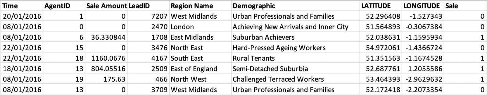
Which contains a mix of Numeric, Categorical and Time based features which are only loosely correlated. In most cases
there is an upper bound on how many observations we have available (in this case since each observation was generated by a physical action
of a sales person calling a potential customer) which tends to fall well short of a million, let alone billions.
These practical realities mean that while Neural Networks are able to far outperform other approaches at the kind of problems they inherently excel at, they can conversely struggle at many common day to day business datasets.
Luckily, Kortical AutoML will figure out when a Neural Network would be the best approach, and design the architecture and tune the hyper parameters to get the best results from it.
We typically find Neural Networks do well when we have a large number of a consistent column types such as:
- Text or high cardinality categorical inputs, but not lots of other column types
- Time series with lots of lagged variables
- Arrays of sensor or machine data data
Neural networks are also a great choice if you need a smooth decision boundary.
Note
The word2vec text embedder is itself a kind of Neural Network, which will be automatically combined with other model
types to get the best of both worlds where applicable. This gives the advantages of a Neural Network for the text columns, while using a
more suitable model type to interpret this and combine with the rest of the features.
Available Parameters: Deep Neural Network Classifier
- deep_neural_network:
  - number_of_hidden_layers
  - hidden_layer_width
  - hidden_layer_width_attenuation
  - activation
  - alpha
  - max_iter
  - solver
  - beta_1
  - beta_2
  - epsilon
  - batch_size
  - shuffle
  - learning_rate_init
  - early_stopping
  - tol
  - validation_fraction
Available Parameters: Deep Neural Network Regressor
- deep_neural_network:
  - number_of_hidden_layers
  - hidden_layer_width
  - hidden_layer_width_attenuation
  - activation
  - alpha
  - max_iter
  - solver
  - beta_1
  - beta_2
  - epsilon
  - batch_size
  - shuffle
  - learning_rate_init
  - early_stopping
  - tol
  - validation_fraction
  - verbose
  - warm_start
# Linear Models
Linear models (Linear (opens new window) or Logistic (opens new window)
regression in the regression and classification cases respectively) assume a linear relation between the input features
and the target variable. In cases where this is true
(or mostly true), they are one of the more powerful yet most underrated Machine Learning approaches. Linear models
are quick to train, transparent to interpretation and inherently harder to overfit than their non-linear brethren. They are also able
to handle larger and sparser input feature spaces very well compared to Forest based approaches.
Due to their nature they are never going to be able to capture non-linearity in the data, so could be wholly unsuitable to some problems. It is often not easy to determine up front where this might be the case, so the initial models explored by the Kortical platform always include a linear model to test if this is the case.
We find that linear models will tend to be the best approach in situations where:
- We have a high dimensional, sparse, input, (when we have lots of text or high cardinality categorical features for example.)
- The input contains transformed features which capture the non-linear elements (so the model itself can be linear).
- We want a smooth decision boundary.
Conversely, we don't see them at their best when:
- We have dense features with complex interactions which need to be uncovered.
- We have XOR like relationships between input features (or any other interactions impossible to express with a linear boundary).
Available Parameters: Linear Classifier (Logistic Regression)
- linear:
  - C
  - class_weight
  - max_iter
  - tol
  - multi_class
  - solver
  - penalty
  - dual
  - fit_intercept
  - intercept_scaling
Available Parameters: Linear Regression
- linear:
  - fit_intercept
  - normalize
  - copy_X
# Support Vector Machines
Support Vector Machines (SVMs) (opens new window) are like Linear Models in the sense that they attempt to find a line (or hyperplane) that best separates input classes. However, unlike Linear Models they are able to describe non-linear relationships by projecting input points into a higher dimensional space where inputs become linearly separable (using an efficient method known as the Kernel trick).
SVM's are the only algorithm that Kortical AutoML does not try by default. This is due to scaling issues with respect to the input observations, the difficulty they have with several common problem types (especially where classes are noisy or not well separated) and the fact they do not produce output probabilities by default, requiring an expensive extra step at predict time to create them.
However, they can be very effective in certain situations:
- Certain types of high dimensional problem, especially cases in which you have a high number of input dimensions but low numbers of observations (which most other models struggle with).
- Cases where classes are nicely separable and there is not much noise.
Available Parameters: SVM Classifier
- svm:
  - C
  - kernel
  - shrinking
  - tol
  - epsilon
  - verbose
  - max_iter
  - gamma
Available Parameters: SVM Regressor
- svm:
  - C
  - kernel
  - shrinking
  - tol
  - epsilon
  - verbose
  - max_iter