Model Exploration

When you click Explore on a model you will be taken to the model exploration section for that model.

Model Scores

At the top of the model exploration you will see a table containing the Model Scores as can be seen below

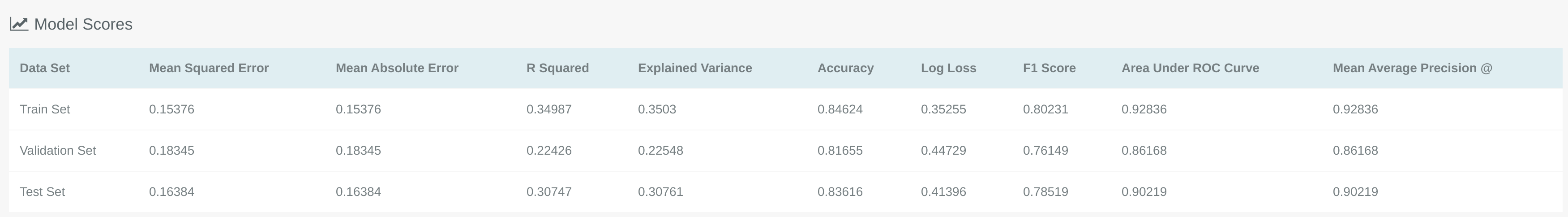
This table shows you the scores this model achieved on the test, train and validation sets for each metric type that is supported.

Threshold Explorer

The threshold explorer gives users the ability to see the effect that changing the threshold value has on the accuracy, precision and recall for that model.

Note

The threshold explorer will only be displayed for binary classification and multi-label classification models.

Test Set

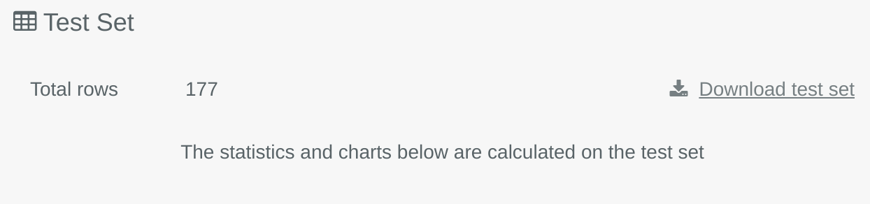
This area of the model explore gives you the ability to download the test set that was used to get the scores shown in the Model Scores table. This test set is used to calculate the scores in the ROC chart, confusion matrix and the F1-Score table.

ROC Chart

Binary Classification

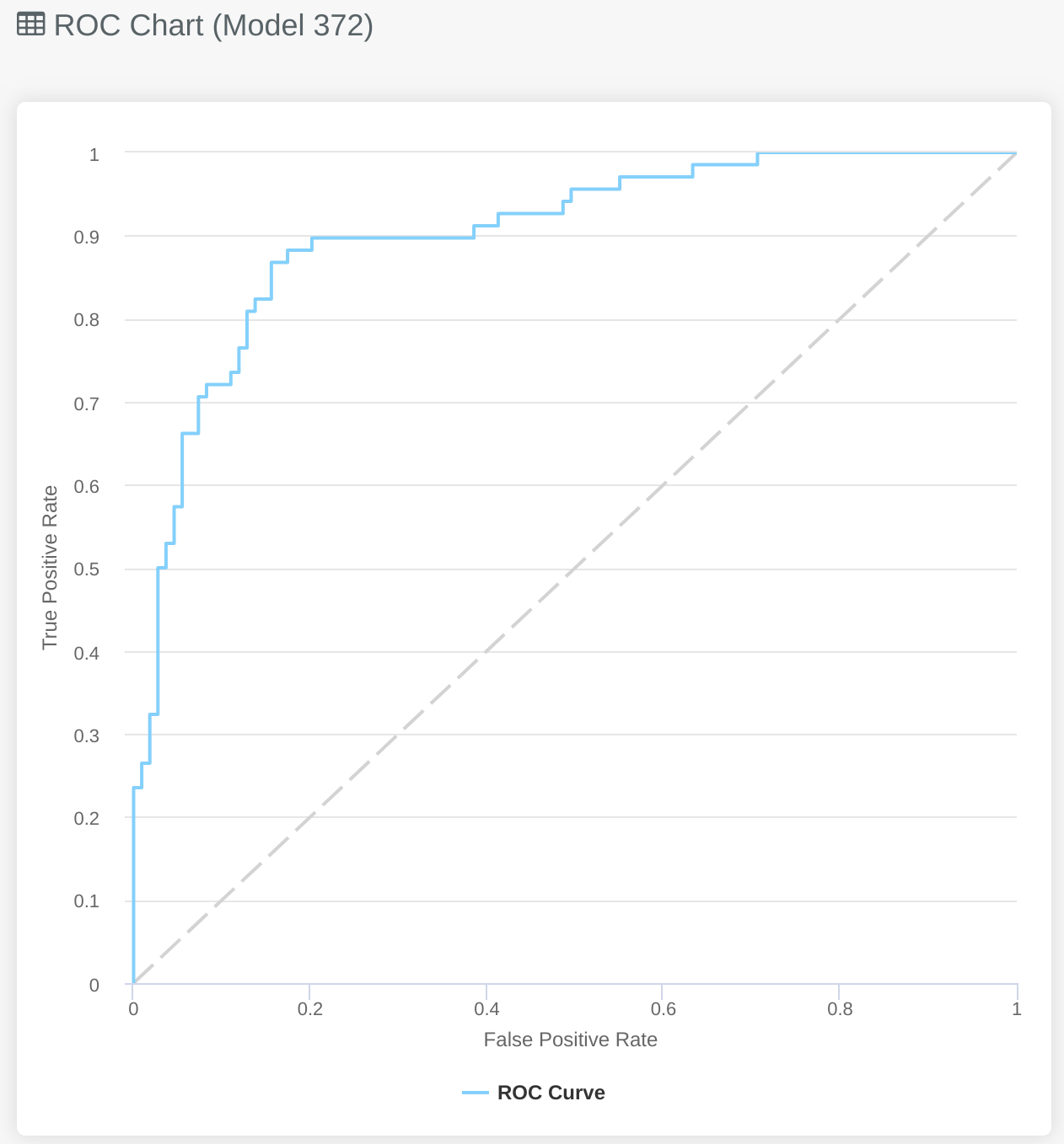
The ROC Chart shows the trade-off between false positives and true positives across the full range of classification thresholds. It does this by plotting the true positive rate vs the false positive rate.

Multi-label Classification

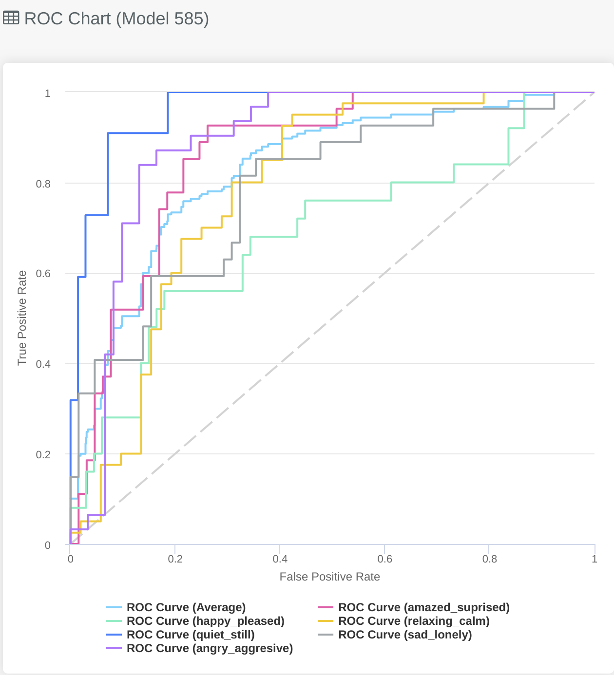
The ROC chart for multi-label classification problems will look slightly different to the binary classification problems, this is because it gives you an overview of how the model does for each specific label, as well as how it performs on average over all labels. To enable and disable the different lines for each label you can click on the key at the bottom of the graph. In this example you might be particularly interested in identifying which Twitter users are predicted to be sad_lonely and as a result reach out to them to see if they need any support.

Multiclass Classification

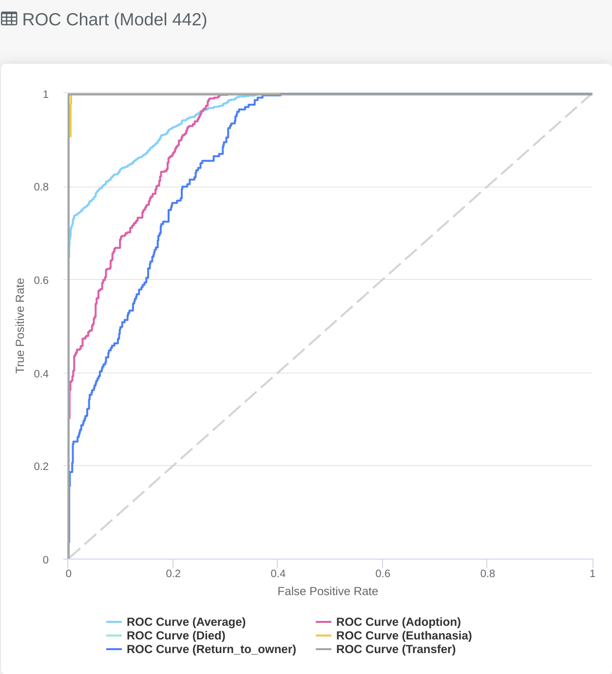
Similar to the Multi-label graph described above the Multiclass ROC chart gives you an overview of how the model performs for each class. We can see the light blue line is the average performance of the model across every class. The lines in the graph that show a perfect AUC curve also help to identify issues in the dataset (as a perfect prediction on the training set is something worth investigating) e.g. leaky features, or few examples in the training data.

Predicted vs Actual

Regression

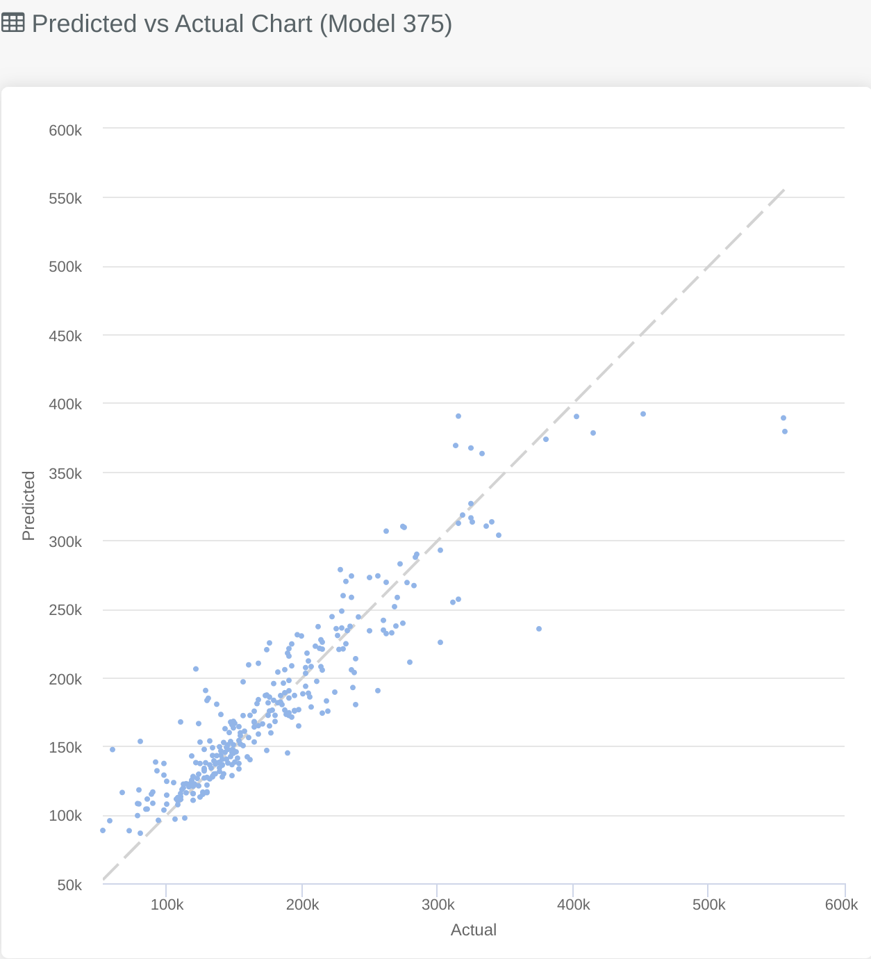
In the same place you would see the ROC Charts mentioned above you will find the predicted vs actual chart for regression problems. This gives you an overview of where the model struggles over the problem domain, by clearly visualising where the predicted and actual are closely matched and where they differ.

The closer to the central diagonal line the points on the graph are the better the model will be. In the graph above you can see an example from predicting house prices.

The majority of the training data is on the lower end of the scale as there is a large cluster of points in the bottom left of the graph, whereas when the price increases we see the models performance drops off and there are fewer points. This is likely because the majority of the training data is for house prices on the lower end of the scale, adding more training data with more expensive houses would help the model to perform better in that area.

Confusion Matrix

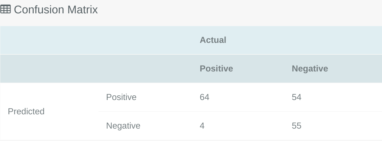
The Confusion Matrix can be used to see the performance of a classification model, it plots predicted values vs actual values and allows an intuitive way to view where the model gets things right and where it gets them wrong. In the image above you can see that this particular model correctly predicted 64 positive cases that were positive, and incorrectly predicted 4 cases as positive which were actually negative. Depending on your problem type the importance of false positive vs false negatives may vary, so you can use this table to ensure that the model you have selected fits the problem domain.

TIP

By adjusting the classifier threshold inside the Threshold Explorer you can see how the confusion matrix would change with different thresholds.

F1 Score Table

Binary Classification

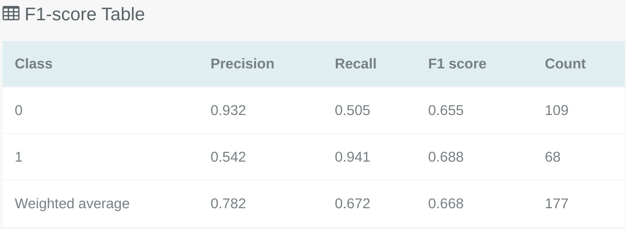
The F1 Score table shows the Precision, Recall and F1 scores for each class in the classification problem. Like the Confusion Matrix this can also be used in combination with the Threshold Explorer to see how the F1 scores would change if different thresholds were applied to the model.

Multi-label Classification

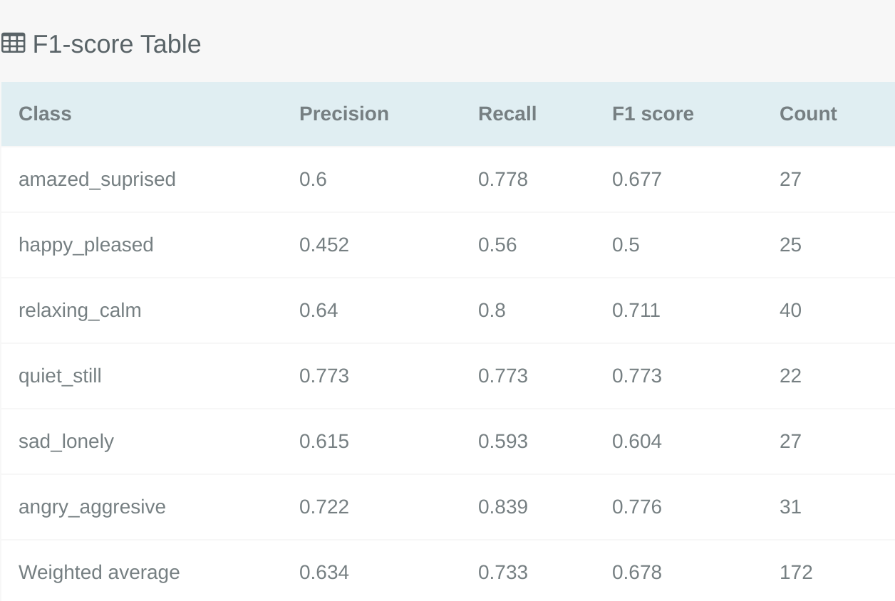
The F1 Score table for multi-label classification will differ slightly to the binary classification F1 table described above, this is because it shows the F1 score for each specific label in the problem.

Multiclass Classification

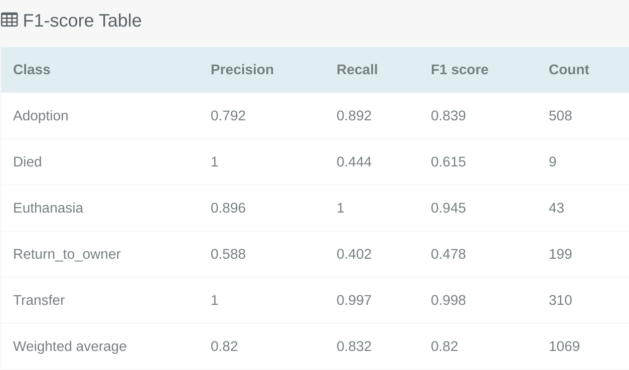
Similar to the multi-label classification F1 Score table the multiclass F1 Score table will show a break down of the F1 Score for each class. This gives the opportunity to pick a model which performs well on the most important classes for your problem type.

Model Code

To see the original and expanded code of this specific model you can click on the code tab seen below:

Original Specification

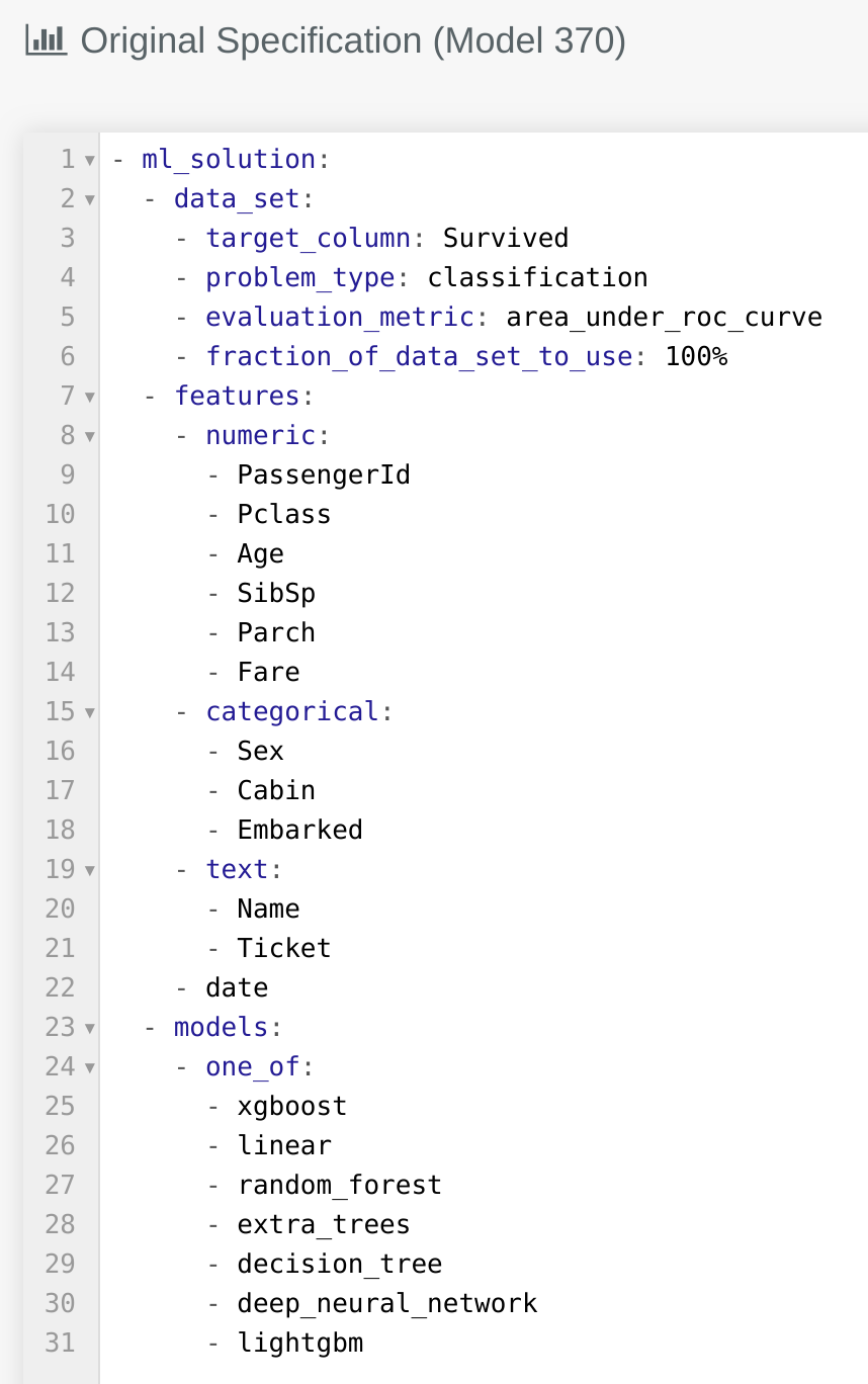
The original code shows what code was submitted on the lab page, as defined with the Kortical language, at the start of the AutoML train that produced this model. It outlines the search space of the AutoML solution for this train. By comparing it to the expanded code below, we can see where this specific machine learning solution (ML solution) fits within this search space.

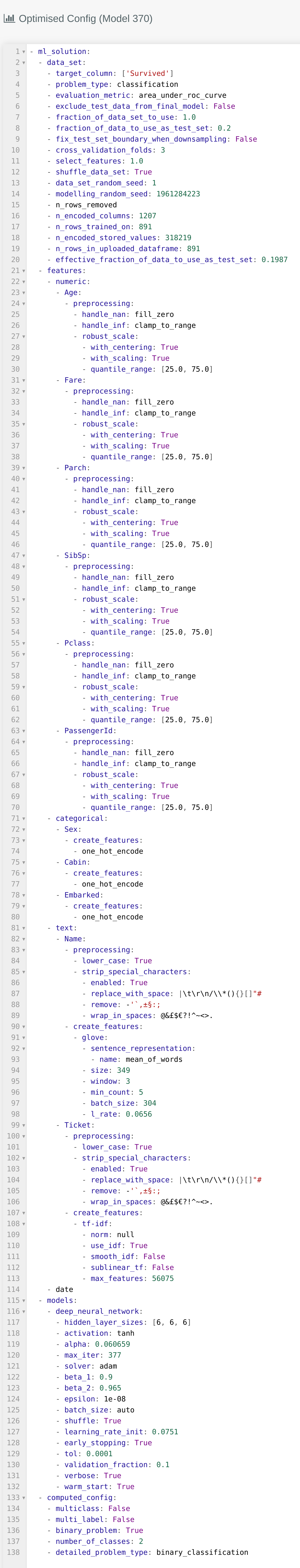
Optimised config

The optimised configuration is the expanded code used for this specific machine learning solution. All of the blanks in the original code have been filled in by the AutoML as part of its intelligent search. It represents a single point in the search space. By using this code, you have enough information to fully re-create the machine learning solution itself outside of the Kortical platform.

An example optimised config can be seen below:

More detail on each of the sections in the code can be found here.

TIP

You can copy the optimised config into your lab page to recreate the same model. If you were to remove some parameters you would allow the machine learning solution to vary in that space. e.g. You could remove the section specifying -deep_neural_network and this would keep all the above specified preprocessing and feature creation steps but allow the specific model type to vary.